Stock Price Forecasting With Machine Learning: Getting Started

In this series, we focus on stock price forecasting using machine learning techniques. Every machine learning problem consists of three fundamental components:

1. Data with Features: The input variables (features) used to make predictions
2. Model: The algorithm that learns patterns from the data (e.g., linear regression, neural networks)
3. Objective Function: The metric we optimize (e.g., mean squared error, R²)

However, stock price data is time series data, which behaves fundamentally differently from typical machine learning datasets.

Why Time Series Data is Different

Most machine learning assumes data points are independent and identically distributed (i.i.d.). For example, images in a classification dataset are usually independent of each other.

Time series data violates this assumption:

• Sequential dependence: Today’s price depends on yesterday’s price
• Temporal ordering matters: We cannot randomly shuffle observations
• Non-stationarity: Statistical properties may change over time

These characteristics require different techniques for:

• Data preprocessing and feature extraction
• Model selection
• Loss function evaluation

Let’s explore these through a simple practical example.

Loading Stock Price Data

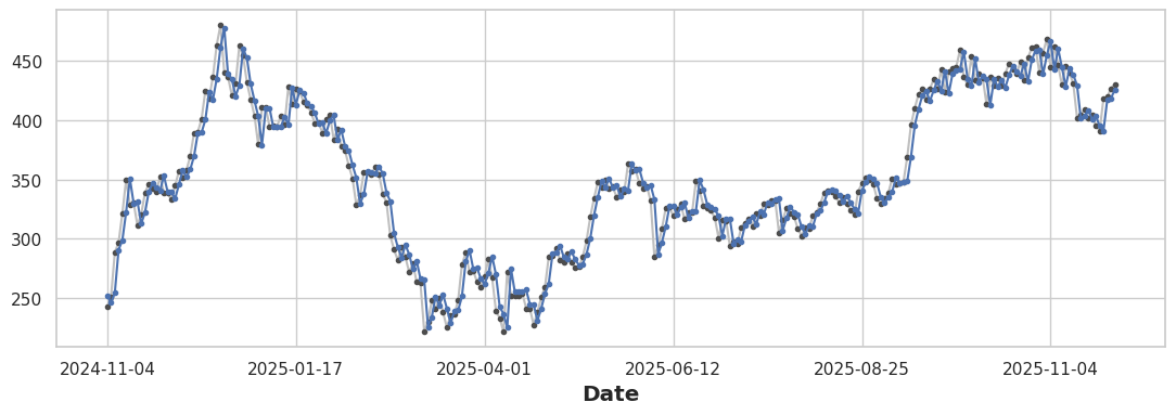
We’ll use Tesla (TSLA) closing prices from November 2024 to November 2025. The yfinance library can download historical stock data; here we assume it’s already saved as stock_data.csv:

import pandas as pd
import numpy as np
from sklearn.linear_model import LinearRegression
from sklearn.metrics import r2_score, mean_absolute_error
import matplotlib.pyplot as plt

# Configure plot styling
plt.rc("figure", autolayout=True, figsize=(11, 4), titlesize=18, titleweight="bold")
plt.rc("axes", labelsize="large", labelweight="bold", titlesize=16, 
       titleweight="bold", titlepad=10)

# Load and prepare data
df = pd.read_csv('stock_data.csv', 
                 parse_dates=['Date'],
                 index_col='Date',
                 usecols=['Date', 'Close', 'Asset'])
df = df[df['Asset'] == 'TSLA'].drop(columns=['Asset'])

df.head()

Output:

Date	Close
2024-11-01	248.979996
2024-11-04	242.839996
2024-11-05	251.440002
2024-11-06	288.529999
2024-11-07	296.910004

Baseline: Linear Regression with Time Index

Let’s start with the simplest approach: feeding raw time information into linear regression. We create a time dummy feature - just a counter from 0 to n-1:

# Create time feature
df['Time'] = np.arange(len(df.index))

# Fit linear regression
X = df[['Time']]
y = df['Close']

model = LinearRegression()
model.fit(X, y)
y_pred = pd.Series(model.predict(X), index=X.index)

# Visualize
fig, ax = plt.subplots()
ax = y.plot(style='o-', color='0.75', markersize=4, 
           markerfacecolor='0.3', markeredgecolor='0.3')
ax = y_pred.plot(ax=ax, linewidth=3)
ax.set_title('TSLA Closing Prices - Time Feature Only')

Result: We get a straight line! This captures the long-term trend but misses all the day-to-day fluctuations. The model learns: Price = weight × Time + bias, which can only represent linear trends.

This is where feature engineering becomes critical.

Feature Engineering: Introducing Lag Features

Key insight: In stock prices, yesterday’s price is highly correlated with today’s price. We can leverage this serial dependence by creating lag features.

A lag feature shifts past values forward in time:

# Create 1-day lag feature
df['Lag_1'] = df['Close'].shift(1)

df.head()

Output:

Date	Close	Time	Lag_1
2024-11-01 00:00:00-04:00	248.979996	0	NaN
2024-11-04 00:00:00-05:00	242.839996	1	248.979996
2024-11-05 00:00:00-05:00	251.440002	2	242.839996
2024-11-06 00:00:00-05:00	288.529999	3	251.440002
2024-11-07 00:00:00-05:00	296.910004	4	288.529999

Note the first row has NaN since no prior observation exists.

Why lag features? Let’s visualize the correlation:

# Remove NaN values
df_lag = df.dropna()

# Lag plot - shows correlation between consecutive days
fig, ax = plt.subplots()
ax.plot(df_lag['Lag_1'], df_lag['Close'], '.', color='0.25')
ax.set_xlabel('Lag_1')
ax.set_ylabel('Close')
ax.set_title('Lag Plot with Linear Regression Fit')
ax.set_aspect('equal')

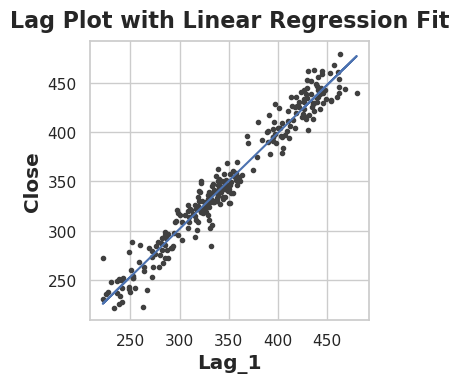
The strong linear relationship confirms that yesterday’s price is an excellent predictor of today’s price. This serial dependence means we can use past values to forecast future values - a key characteristic of time series data.

Training with Lag Features

Now let’s train a model using only the lag feature:

# Fit model with lag feature
X = df_lag[['Lag_1']]
y = df_lag['Close']

model = LinearRegression()
model.fit(X, y)
y_pred = pd.Series(model.predict(X), index=X.index)

# Visualize predictions over time
fig, ax = plt.subplots()
ax = y.plot(style='o-', color='0.75', markersize=3, 
           markerfacecolor='0.3', markeredgecolor='0.3')
y_pred.plot(ax=ax, color='C0', style='o-', markersize=3, 
           markerfacecolor='C0', markeredgecolor='C0')

The Shadow Effect: Why Lag Alone is Insufficient

Observation: The prediction curve follows the actual prices almost perfectly, but is shifted one step behind - like a shadow!

Why? The model learns: Today's Price ≈ Yesterday's Price. So:

• Prediction at day t = f(Actual at day t-1)
• The prediction curve is just yesterday’s actual curve

This isn’t traditional overfitting - it’s the inherent limitation of using only lag features. While the lag captures short-term momentum (day-to-day persistence), it:

• Cannot anticipate direction changes
• Misses the underlying trend
• Acts as a naive “repeat yesterday” forecast

Combining Long-Term and Short-Term Patterns

The solution: combine time features (long-term trend) with lag features (short-term momentum):

# Create combined features
df['Time'] = np.arange(len(df.index))
df['Lag_1'] = df['Close'].shift(1)
df_combined = df.dropna()

# Fit model with both features
X = df_combined[['Time', 'Lag_1']]
y = df_combined['Close']

model = LinearRegression()
model.fit(X, y)
y_pred = pd.Series(model.predict(X), index=X.index)

# Visualize
fig, ax = plt.subplots()
ax = y.plot(style='o-', color='0.75', markersize=3, 
           markerfacecolor='0.3', markeredgecolor='0.3')
y_pred.plot(ax=ax, color='C0', style='o-', markersize=3, 
           markerfacecolor='C0', markeredgecolor='C0')

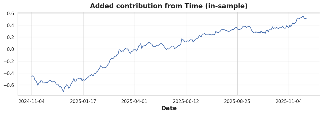
The combined model captures both patterns. To isolate the time feature’s contribution:

# Lag-only predictions
X1 = df_combined[['Lag_1']]
m1 = LinearRegression().fit(X1, y)
pred_lag = pd.Series(m1.predict(X1), index=df_combined.index)

# Time + Lag predictions
X2 = df_combined[['Time', 'Lag_1']]
m2 = LinearRegression().fit(X2, y)
pred_both = pd.Series(m2.predict(X2), index=df_combined.index)

# Plot the difference
(pred_both - pred_lag).plot(title="Added contribution from Time (in-sample)")

Evaluating with Objective Functions

We measure performance using two metrics:

• R² (coefficient of determination): Proportion of variance explained (higher is better, max = 1)
• MAE (mean absolute error): Average prediction error in dollars (lower is better)

print("Lag-only:", r2_score(y, pred_lag), mean_absolute_error(y, pred_lag))
print("Combined:", r2_score(y, pred_both), mean_absolute_error(y, pred_both))

Output:

Lag-only: 0.9545711149515113 10.630869656770322
Combined: 0.9546014062251829 10.61683874699556

The improvement is small because lag features already capture most of the predictable pattern. However, the time feature adds the directional bias needed for trend-following.

This is the first article in a series on stock price forecasting. Next, we’ll explore multi-lag features, moving averages, and more sophisticated models.